1. Calculate the Total
2. Calculate the Average.
3. Calculate the Highest & Lowest Marks in every subjects
4. The Result should be pass if the students get 35 or > than 35 marks in each subject5. The sheet should be rename as “Mark list of 2005-06”
Solution:
Total : =SUM(B4:D4)
AVERAGE : =AVERAGE(B4:D4)
HIGHEST : =MAX(B4:B12)
LOWEST : =MIN(B4:B12)RESULT : =IF(MIN(B2:D2)>=35,”PASS”,”FAIL”)
1. Calculate the Total & Average sales.
2. The comment should be “Good Sale” if the average sales are above Rs.35000/- otherwise
the comment should be “Improving Sales”.3. The sheet should be renamed as “Quarterly sales for 95-96”.
Solution:
Total : =SUM(B4:E4)AVERAGE : =AVERAGE(B4:E4)COMMENT : =IF(G2>35000,”GOOD SALE”,”IMPROVING SALE”)Right click on sheet and select the Rename option for rename the sheet
1. Calculate the Total & Average sales of every salesman.2. The Commission shall be calculated as 15% of average sale. If the average
sale is less than 4000 then “No commission”.
Solution:
Total : =SUM(B4:D4)AVERAGE : =AVERAGE(B4:D4)COMMISSION: =IF(F2>4000,F2*15%,”NO COMMISSION”)
1. Calculate Total variable expenses.2. Calculate Gross profit as=Sales-Total variable expenses.3. Calculate Total fixed expenses.4. Calculate Profit before tax as = Gross profit – Total fixed expenses5. Calculate Tax as 20% of profit before tax.6. Calculate Net profit = Profit before tax – Tax.
Solution:
Total variable expenses : =SUM(B7:B9)Gross profit : =B4-B10Total fixed expenses : =SUM(B14:B17)Profit before tax : =B11-B1820% TAX : =B19*20%Net Profit : =B19-B20
1. Calculate the Interest at 23% on Loan amt. (use absolute reference)2. Rename the sheet as “Calculation of interest amount”.
Solution:
Interest : =B4*E3(Press F4 function key)Right click on sheet and select the Rename option for rename the sheet
1. Calculate the Discount Amt. 20% on Seasonal Sale2. Calculate the Collection
Solution:
Discount : =C4*F3(Press F4 function key)Collection : =B4-C4
1. Calculate HRA as =10% of basic salary2. Calculate DA as = 15% of basic salary3. Calculate CONVEYANCE as = 5% of basic salary4. Calculate Total = BASIC + HRA + DA + CONV.5. Calculate PF as = 5% of TOTAL6. Calculate Net Salary = TOTAL-PF7. Calculate Designation as = if the employees net salary is more than 5000/- hisDesignation is Executive otherwise he is a Clerk.8. Rename the sheet to “Payroll”.
Solution:
HRA : =B4*10%DA : =B4*15%CONVEYANCE : =B4*5%TOTAL : =SUM(B4:E4)PF : =F4*5%NET SALARY : =F4-G4DESIGNATION : =IF(H2>5000,”EXECUTIVE”,”CLERK”)
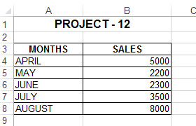
Create a Column chart for the above data with details
Solution:
First select the Table from A3 to B10, then insert chart from Insert-2D Column Chart option or from Chart button from Insert Tab. Then give Axis Titles, Legents, Data Labels for chart.
Sort the table data Name wise, Product wise then apply Sub Total for table and Filters
Solution:
1. Select the table from A3 to D16 then select Sort option from Data Tab =>Sort by=>City then OK2. Sub Total : Select the table from A3 to D16 then select Subtotal option from Data Tab =>At each change in =>CityUse Function=>Sum
Add subtotal to =>Sales Value3. Filter : Click at the header of the table then select Filter option from Data Tab
Calculate the No. of Days and Fine Status from the above Table
Solution:
No. of Days : =D4-C4Fine Status : =IF(E2>15,(E2-15)*5,”NO FINE")
Calculate the Discount Card for above Sales Report
Solution:
=IF(B2>=90000,”GOLD CARD”,IF(B2>=80000,”SILVER CARD”,IF(B2>=65000,”ALUM CARD”,IF(B2>=50000,”PLATINUM CARD”,”NO CARD"))))
Copy the the above table in other software like Word, Power Point etc.
Solution:
1. Select the table from A3 to B8 then select Copy option from Home Tab2. Open Power Point then click on Arrow near Paste option =>Paste Special=>Paste Link=> Microsoft Excel 2003 Worksheet Object =>ok
DATA VALIDATION
For Date - Select E2 to E14 range then click on the Data Tab → Data Validation→ Setting
For List creation - First type a City names in a new cell to create a new list
Then Select B2 to B14 range then click on the Data Tab → Data Validation→ Setting
Finally Select City from the list
What If Analysis
Goal Seek : To set a target value for any table, click on Data → What if Analysis →
then select Goal Seek option
select the Set Cell-E9, To Value-30000 and By changing-E7 cell shown in below:
Scenario Manager : To show the changing value of a table, click on Data → What if Analysis →then select Scenario Manager
Date and Time Functions
1 : =NOW()2 : =TODAY()3 : =DATE(2021,7,10)4 : =DAYS360(C8,C9,TRUE)5 : =YEARFRAC(C8,C9,3)
6 : =DATEDIF(C12,TODAY( ),"Y")
7 : =DAY(C3)8 : =MONTH(C3)9 : =YEAR(C3)10 : =HOUR(C3)11 : =MINUTE(C3)12 : =SECOND(C3)13 : =NETWORKDAYS(B21,B22,B23)14 : =NETWORKDAYS.INTL(B26,B27,11,B28)


